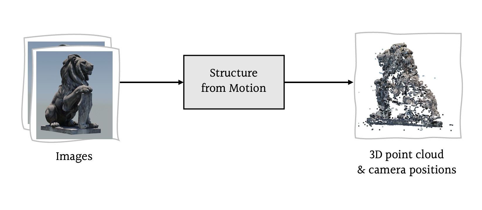
3D reconstruction is a central problem in computer vision, focused on inferring three-dimensional structures from a collection of two-dimensional images. One popular approach to this problem is to simultaneously infer the camera motion (position and orientation) and scene structure (as a point cloud), a class of methods known as Structure from Motion—or SfM for short.
For my third year dissertation project at the University of Cambridge, I implemented and evaluated a complete SfM pipeline, focusing on how alternate approaches to two stages in particular—triangulation and bundle adjustment—affected the reconstruction accuracy.
What is Structure from Motion?
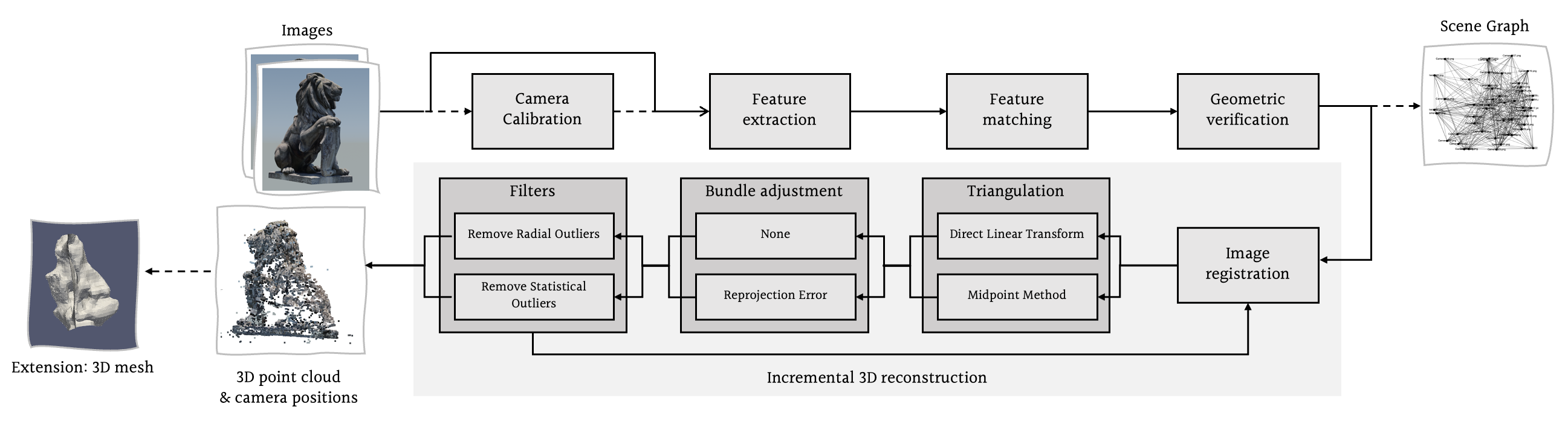
Structure from Motion consists of several stages, as outlined below:
- [Optional] Camera Calibration — accounts for camera-specific parameters such as focal length and optical centre.
- Feature Extraction — identifies distinctive features, or 'key points', in each image.
- Feature Matching — identifies occurrences of the same feature in different images.
- Geometric Verification — prunes geometrically implausible feature matches.
- Image Registration — estimates the pose of the camera at the moment it captured a given image.
- Triangulation — calculates the 3D position of a key point in the scene based on its position in multiple images.
- [Optional] Bundle Adjustment — jointly refines all camera poses and 3D scene points estimated thus far.
- [Optional] Filtering — removes outlier scene points.
Calibrating the Camera
The mathematical operation underpinning photography is a projection: we take a 3D scene, which contains some scene points $\mathbf{X}$, and, by projecting these points onto a plane, obtain some 2D image points $\mathbf{x}$: $$\mathbf{\hat{x}} = K\begin{bmatrix} R & \mathbf{t} \end{bmatrix}\mathbf{X}$$ What Structure from Motion aims to estimate is essentially the reverse transform that maps 2D image points back to their original 3D scene points. For a single image, this is infeasible due to loss of depth information in the projection; however, by identifying common points across multiple images, we can infer not only the positions of the 3D scene points but also the positions of the cameras themselves.
Camera calibration is the process of estimating a camera's so-called intrinsic parameters; these are camera-specific measurements such as its optical centre and focal length, which can lead to distortion in the captured images.
The intrinsic parameters are represented by $K$: $$K = \begin{bmatrix}f_x & s & c_x \\ 0 & f_y & c_y \\ 0 & 0 & 1\end{bmatrix}$$ in which $(c_x, c_y)$ is the optical centre, $(f_x, f_y)$ is the focal length, and $s$ is the skew coefficient. These parameters can be estimated by taking multiple photographs of a known calibration image (a chess board, for instance) with the same camera.
Extracting Features
Feature extraction finds, for each input image $I_i$ (where $i = 1, \dots, N_I$), a set $\mathcal{F}_i = \{ (\mathbf{x}_j, \mathbf{f}_j) \mid j = 1, \dots, N_{F_i} \}$ of distinctive visual features in that image. Here, $\mathbf{x}_j$ is the key point—that is, the feature's location in the image coordinate space—while $\mathbf{f}_j$ is a descriptor of the feature's appearance.
These key points can be used to identify alignments between images - for example, if a pair of images show the same scene from two different angles. We will do this by searching for similar feature descriptors across images; an 'ideal' feature descriptor is therefore one that is invariant to scale, orientation, and lighting conditions. One feature descriptor that satisfies these criteria is the Scale-Invariant Feature Transform (SIFT), which is the one I used in this project.
Finding Feature Matches
Feature matching finds a matching between two sets of features $\mathcal{F}_i$ and $\mathcal{F}_j$ by comparing feature descriptors. The brute force approach would be to perform this search on each pair of images $(I_i, I_j)$, such that $i < j$, with a total time complexity of $O(N_I^2 N_{F_i}^2)$. The output of this stage is an $N_I \times N_I$ matrix of feature matches $\mathcal{M}$, in which each entry $\mathcal{M}_{ab} \in \mathcal{F}_a \times \mathcal{F}_b$ represents the matches between images $I_a$ and $I_b$.
$\mathcal{M}_{ab}$ is a solution to what is called the correspondence problem, meaning it represents a set of points in one image and their corresponding points in another image; each such pair of 2D image points in this set can be used to reconstruct a single 3D scene point.
Verifying Geometric Consistency
Features are matched based only on similarity of appearance descriptors, which tends to yield some false positives. This is particularly problematic when images contain repetitive features, as shown below; two points in the left image correspond to a single point in the right image, because they all have a similar appearance.
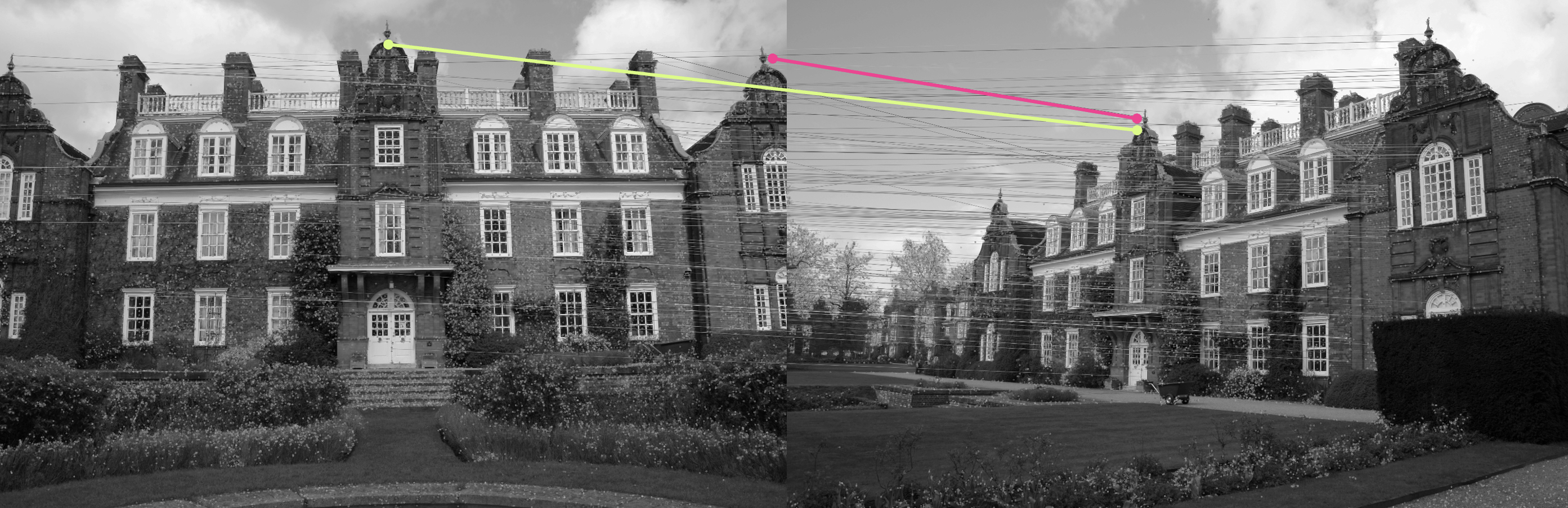
Fortunately, these false feature matches can be identified and pruned through a process called geometric verification, which defines a geometric transformtion between the images.
Specifically, for uncalibrated cameras $I$ and $I'$, we wish to find the fundamental matrix $F$ which satisfies the constraint $\mathbf{x'}^\top F \mathbf{x} = 0$, for all pairs of corresponding keypoints $(\mathbf{x}, \mathbf{x'})$, expressed in homogeneous image coordinates.
Alternatively, for calibrated cameras (for which the intrinsic matrix $K$ is known), we estimate the essential matrix $E = (K')^\top F K$, which satisfies $\mathbf{y'}^\top E \mathbf{y} = 0$, for all pairs of corresponding keypoints $(\mathbf{y}, \mathbf{y'})$, expressed in homogeneous, normalised image coordinates.
In either case, this boils down to applying the epipolar constraint: for any point $\mathbf{x}$ in the first image, its match $\mathbf{x'}$ in the second image is constrained to lie on the epipolar line, $\mathbf{l'} = F \mathbf{x}$—and vice versa. A feature correspondence that satisfies this condition (within some margin of error) is considered geometrically plausible; other feature correspondences are discarded.
Image Registration
Image registration is the process of estimating the pose of the camera at the moment it captured a particular image. The pose is represented as a $3 \times 4$ matrix $[R \mid \mathbf{t}]$ (called the extrinsic matrix), where $R$ and $\mathbf{t}$ are the camera's rotation and translation, respectively.
On the first iteration, the scene reconstruction is initialised by registering a pair of cameras simultaneously. The positions of these cameras (relative to each other) is derived from their keypoint correspondences, a relationship represented via the essential matrix $E$.
Subsequent cameras are registered one at a time using feature matches between the new image and images that have already been 'registered' within the reconstruction; this is known as the Perspective-n-Point (PnP) problem.
Triangulation
Triangulation is the process of determining the location of a 3D scene point $\mathbf{X}$ from its measured image points $\mathbf{x}$ in more than one image. The scope of this project was limited to two-view triangulation methods—that is, those that consider a pair of image points $(\mathbf{x}_1, \mathbf{x}_2)$ from two different camera views.
To triangulate a scene point, we first assume knowledge of the $3 \times 4$ extrinsic matrix $[R \mid \mathbf{t}]$ and the $3 \times 3$ intrinsic matrix $K$ for each camera, calculated in the camera calibration and image registration stages, respectively. We then combine these into a single $3 \times 4$ projection matrix $P = K [R \mid \mathbf{t}]$.
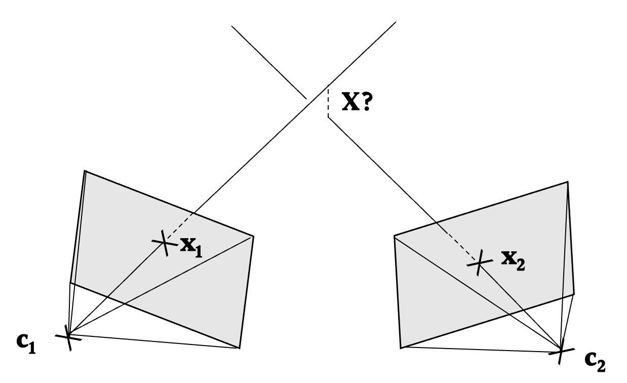
If we assume exact knowledge of these camera matrices and measured image points, the solution to the triangulation problem is trivial: the triangulated scene point $\mathbf{X}$ solves $\mathbf{x}_1 = P_1 \mathbf{X}$ and $\mathbf{x}_2 = P_2 \mathbf{X}$; in other words, $\mathbf{X}$ is the point of intersection of the two backprojected rays, as pictured above.
However, such an assumption is unrealistic. In practice, these backprojected rays are almost always skew. The problem is to therefore find a scene point that 'best fits' the measured image points. There are many ways to do this, but, for my project, I implemented and compared two triangulation methods: midpoint triangulation and linear triangulation.
Bundle Adjustment
The next step of the pipeline is bundle adjustment (BA). BA refers to the joint refinement of all camera poses and scene points estimated thus far; these are esimated separately in the image registration and triangulation stages, but are closely correlated. Uncertainties in triangulation therefore propagate to the next camera pose estimation, and vice versa. This error accumulates over several iterations and can cause the reconstruction to 'drift' to a non-recoverable state.
Bundle adjustment aims to reduce this scene drift by leveraging the redundancy provided by additional camera poses and scene points calculated in later iterations to refine earlier estimates.
The typical approach is to minimise a cost function that incorporates camera poses and scene points spanning several iterations. In this project, I implemented a cost function that measured the total reprojection error, and used Ceres Solver to minimise this function.
Our reconstruction may contain some outlier scene points; these can be removed by filtering. In particular, I implemented statistical outlier filtering (which removes points whose average distance to their nearest neighbours exceeds a particular threshold) and radial outlier filtering (which removes points with too few neighbours within a given radius).
Links
To find out more, check out:
- The GitHub repository for the project